Understanding Big O Notation

Introduction

Big O Notation is a mathematical notation that describes the behavior of a value (most commonly denoted as n) as it reaches infinity. That's how you'd see it explained in most places. The mathematical explanation aside, there's a nuance in the programming usage of the big O notation. It can be used in both Time Complexity and Space Complexity.

Dictionary

Time Complexity - It's used to describe the amount of CPU resources needed in order to finish evaluating the algorithm in runtime

Space Complexity - It's used to describe the amount of memory resources needed in order to finish evaluating the whole algorithm.

Compile Time - This isn't measured with Big O notation. The compile time is the time where your interpreter/compiler to translates your written code into byte-code/machine code respectively.

A good thing about the fact that compile time evaluations aren't accounted for in sites like LeetCode is that you can do compile time optimizations (mainly in languages like C and C++) in order to do compile time evaluation via features like Constant Evaluations and Constant Expressions.

Runtime - This is the time when the program is being executed after compiling it. LeetCode's Time Complexity performance measurement is based on this exact metric.

Analysis

It's very likely that you've seen this Big O notation graph:

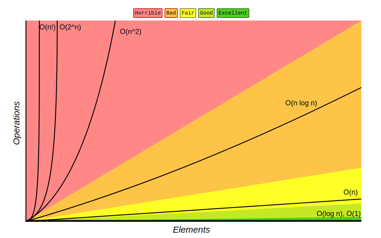
Let's go over these stuff really quickly

• 
  
  Also referred to as constant complexity.
  
  Some of the programming data structures that match this complexity notation are: pushing an item at the front of a vector; looking up an item in a hashed set or a hashed map (dictionary); getting the first element of a singly linked list; getting the last element of a vector.
  
  Not a lot of algorithms are done in this complexity. Usually it's a simple method on a specific data structure.
• 
  
  This is a somewhat common performance region in LeetCode solutions, It's primary use is in Binary Search (Recommended Leets: Palindrome Number and Search Insert Position) This algorithm is common for interview questions and practical to know (and it's also joked that every university student has implemented it).
• 
  
  This is pretty common to see in LeetCode. The concept of it is doing at least one full iteration on your data set. Here's the tricky part though: while removing the last item of a vector is O(1). Removing its first item is actually O(n). You need to do a full traversal from the last item to the first one in order to rearrage all the items properly. Similarly, removing the last item of a singly linked list is also an O(n) operation. You want to be careful with some of the data structures because a mistake like that will easily give insane runtime overhead, turning a viable solution into a bad one.
• 
  
  Usually this is where sorting algorithms fall into, ones like Quicksort (average case... depending on your pivot point... please don't use a pivot point at the end), Heapsort (in every case) and Merge sort (in most cases).
  
  This is for time complexity. The space complexities for Quicksort and Heapsort are O(n log n) best case and O(n) worst case and for Merge sort it's O(n).
• 
  
  A common way to get to this point is doing 2 iterations on your array. (Did I mention how 90% of LeetCode is arrays? Yeah, they're really useful. Anyway). Some problems have O(n²) as the best solutions. Those problems are usually quite rare (At least from my little experience). A more interesting way is matrices. Those big two-dimensional arrays you see in University math classes. They can be coded into a computer too. The syntax is usually arr[i][j] but that's not very important right now. The more important part is that these matrices are traversed in O(n²) time complexity. Also, Bubble sort is a O(n²) algorithm. It's very impractical but it's the easiest sorting algorithm to understand so you should just know it if you've been getting into the more complex ones like Quicksort, Heapsort and Mergesort.
• 
  
  
  Chances are that you've seen this notorious Fibonacci sequence solution. This is a bad solution in practice though. If you refer to the image at the start of this section. It's in the second slowest section. The solutions here (and at O(n!)) consist of brute force algorithms. They only work on small data sets and have an exponential growth in their resource consumption.
• 
  
  Similarly to O(2ⁿ) it's useful in brute force algorithms and actually evaluating n! (n factorial).

Optimizing for memory vs optimizing for space

This depends on a lot of factors. Although this will be the example use case:

Finding prime numbers (credit to b001 on YouTube):

Let's break down the primary three ways of doing it:

1. Trial Division

   The most efficient memory wise. It's the slowest in practice though because it requires you to first: evaluate the square root of every number, second: do modulo division for all the numbers that are less than the square root of that number. How does that even work? This image from the video will help understand just that:

   

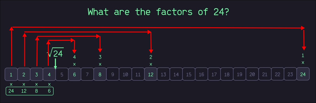
   Interesting right? They're mirrored. That's always the case. The explanation is rather simple: 3² is 9 obviously, so whatever is a divisor of 3 is also a divisor of 9. If this method is applied to an actual prime number here's how it'd look like:

   Let's say 11 is the example. The square root of it is between 3 and 4 (closer to 3) and 4 isn't a prime number either. So all that's needed to get checked is whether 11 is divisible by 2 or 3 (because 4, 6, 8, 10 are already divisible by 2 and 6 and 9 are already divisible by 3 so the math for them would be excessive). Or if you prefer the mathematical explanation:

   if n is divisible by some number p, then n = p × q and if q were smaller than p, n would have been detected earlier as being divisible by q or by a prime factor of q. (Wikipedia)

   The time and space complexities for this algorithm are tricky to explain since they revolve around using square roots, I recommend checking this Wikipedia section if you're interested in the exact details. The only thing that's for sure the case is that Trial division takes less space than both Sieve of Eratosthenes and Dijkstra's approach but it's the slowest one in time complexity.

2. Sieve of Eratosthenes

   This one is the quickest in time complexity of O(n log log n) but it has O(n) memory complexity. The application is pretty simple: get all the numbers from 2 included to n included in an array of boolean values (true by default), then start at 2, go through all multiples of 2 and turn them to false, then do 3 and go through all multiples of 3 (ignoring all already false multiples) and turn them to false. Do that for every number up to n included.

   Despite being O(n) space complexity it also manages to tell you all the prime numbers up to n so it's incredibly efficient in bulk prime number evaluation. In fact it's hands down the best algorithm for that.

3. Dijkstra's Approach

   This one is a bit trickier to explain (you can see this visually at 10:26 from the video) but here's how it goes:

   Unlike the first 2 algorithms this one uses a "pool" and the usual list of prime numbers (where the initial numbers in the pool are also in the prime list). We skip 1 as usual. At 2 we get 2 and it's multiple (4) and add them to the pool as a tuple, then we go to 3, we check the smallest multiple in the pool (4) and if it's larger than our current number (3) we add 3 and its multiple 9 as a tuple of (3, 9) to the pool. The next number is 4, we check the smallest multiple in the pool again, if they're equal then increment the smallest multiple by its associated number. This means that the (2, 4) pair will become (2, 6). Then we go to 5, it's smaller than the smallest multiple so we add it with its multiple in the pool.
   The next one is 6 -> we change the (2, 6) pair to (2, 8).
   7 -> it's smaller than the smallest so we add it to the pool with its multiple.
   8 -> change (2, 8) to (2, 10).
   9 -> change (3, 9) to (3, 12). 10 -> change (2, 10) to (2, 12)
   11 -> Add it to the pool with its multiple

Conclusion

If you only want memory efficiency: do Trial Division.
If you only want speed: use the Sieve of Eratosthenes.
If you want a balance between the two: try out Dijkstra's approach.

As stated in the start of this section. There are a lot of factors to determine when going for memory over speed or vice versa. For example in game development memory efficiency in saving resources for your models is also a speed improvement. The most important factor in determining whether you want to optimize for memory or for speed is the ability to determine what you need more.

The misinformation about big O notation

Big O notation ISN'T the all-be-it in determining whether or not algorithm A is more efficient than algorithm B. There's more to it. The reason is this: Big O notation, as described in the start, is the behavior of a value (n) as it reaches infinity (or in mathematical notation that'd be: n → ∞). This specific notation eliminates all constant values in its determination. This means that O(2n) is portrayed as O(n) (linear), just in the same way that O(1,000n) is portrayed as O(n), so is O(1,000,000n) and so on. The reason for this is because big O notation was meant to only account for the worst case scenario of an algorithm. That worst case scenario being the upper limit of n as it reaches infinity, and because it's only looking at that, it removes all other constants because eventually n will be greater than them. But is this true in practice? In most cases it's not, some of the times you even know your exact data set as well! That means that you can optimize an algorithm based exactly on that data set.

Not only big O

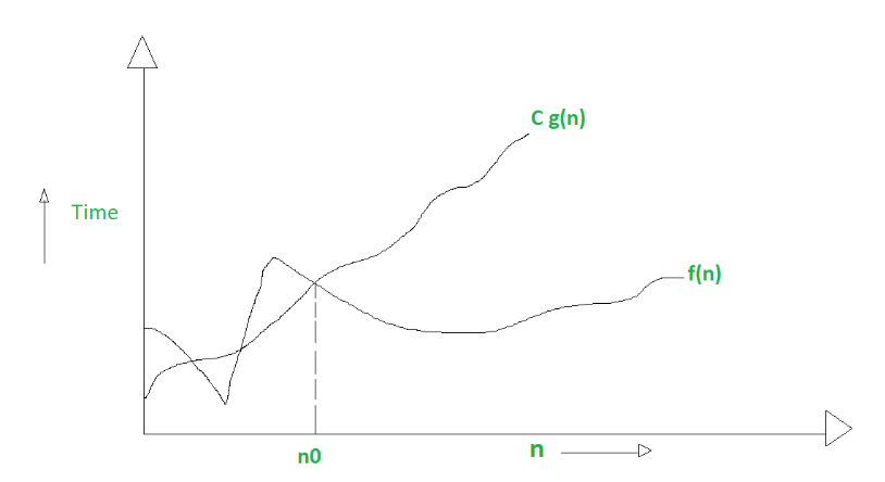
Big O notation describes an algorithm based on its worst case scenario as n grows to infinity. This means it's denoted as this:

0 <= f(n) <= Cg(n) for all n >= n0

Where:

• Everything is greater than or equal to 0
• The running time function that operates on the data set (n) is greater than or equal to 0
• The Constant growth of n is greater than or equal to the f(n)
• The notation applies for every value of n which is greater than n0 (n0 being a positive constant similarly to C).

Credit for all the images in this section
Geeks for Geeks

In this worst case we see how n0 is determined (it takes the highest intersecting point of Cg(n) and f(n)). This eliminates all the quicker to process data sets and only works with the upper bound of n.

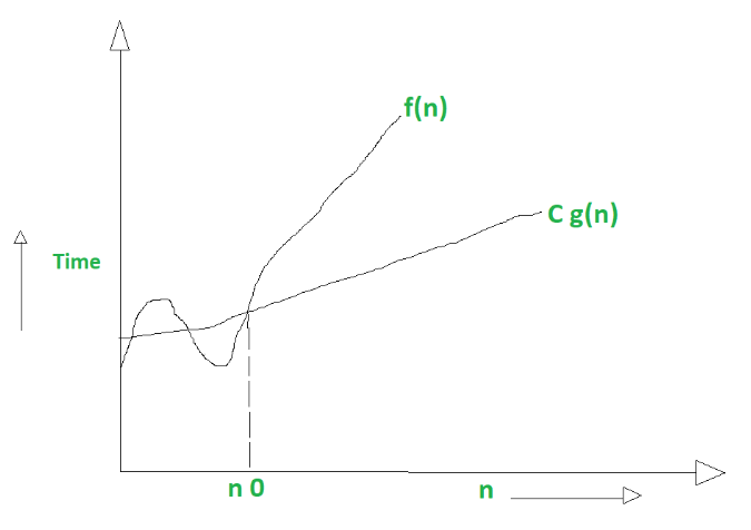
Big Omega (Ω) notation describes an algorithm based on its best case scenario given the lower bound of n. This means it's denoted as this:

0 <= Cg(n) <= f(n) for all n >= n0

Where:

• Everything is greater than or equal to 0
• The Constant growth of n is greater than or equal to 0
• The running time function that operates on the data set (n) is greater than or equal to Cg(n)
• The notation applies for every value of n which is greater than n0 (n0 being a positive constant similarly to C).

Huh? That's quite similar right? Yeah, the constant is just lower here, that's their difference. It can also be equal which makes it compatible with all 3 notation types (oh no that was a spoiler).

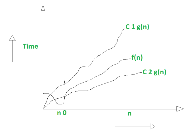
Big Theta (Θ) notation is used to describe the tightest bound between the worst case and the best case scenarios.

0 <= f(n) <= C1g(n) for n >= n0
0 <= C2g(n) <= f(n) for n >= n0

This time we have 2 constants. The 2 equations are the same from the Big O and Big Omega (Ω) notations respectively.
Ultimately we get a merged equation which looks like this:

0 <= C2g(n) <= f(n) <= C1g(n) for n >= n0

Where:

• Everything is greater than or equal to 0
• The Second Constant growth of n is greater than or equal to 0
• The running time function that operates on the data set (n) is greater than or equal to C2g(n).
• The First Constant growth of n is greater than or equal to f(n).
• The notation applies for every value of n which is greater than n0 (n0 being a positive constant similarly to C).

Conclusion

If we simplify it:

Big O is like >=

Big Ω is like <=

Big Θ is like ==

It's not too important to delve so much on the technical details rather than just knowing how the bounds are affected in all of those 3 algorithms. Big O being worst case, Big Ω being best case and Big Θ tightly bounded (evenly distributed) cases.

Summary

The big O notation is a mathematical way to define the worst case scenario performance of an algorithm as its data set reaches infinity. This means it evaluates its performance based on the upper bound of the data set. The performance measured is separated in 2 types: runtime performance (how much your CPU needs to operate on the data set) and memory performance (how much runtime memory your algorithm takes based on your data set). Determining which part of your program you want to optimize depends heavily on your use case. You have to evaluate which one is the better one to optimize for. Also, Big O notation is for the worst case scenarios, there's also Big Ω (Omega) notation for the best case scenarios (where your constant that operates on the data set is less than or equal to your functions input) and a Big Θ (Theta) notation where your growth rate has to be even throughout the growth of your data set. This means that everything that can be described in Big Theta can also be described in Big Omega and Big O notations.